SQL
Frontpage Data visualisation Parametizing data Directory structure R-package SQL Zotero Reproductibility Future endeavours Free research (Machine learning) CV Bibliography
In order to prove my skills in the field of data handling and SQL, this page will show me work with flu data, dengue data and the gapminder data from the {dslabs} package. The flu data and dengue data are both supplied by google, “www.google.org/flutrends AND www.google.org/denguetrends”
First of all, all datasets will be read and inspected in R
#The gapminder dataset
gapminder %>% head()
## country year infant_mortality life_expectancy fertility population gdp continent region
## 1 Albania 1960 115.40 62.87 6.19 1636054 NA Europe Southern Europe
## 2 Algeria 1960 148.20 47.50 7.65 11124892 13828152297 Africa Northern Africa
## 3 Angola 1960 208.00 35.98 7.32 5270844 NA Africa Middle Africa
## 4 Antigua and Barbuda 1960 NA 62.97 4.43 54681 NA Americas Caribbean
## 5 Argentina 1960 59.87 65.39 3.11 20619075 108322326649 Americas South America
## 6 Armenia 1960 NA 66.86 4.55 1867396 NA Asia Western Asiadengue<-read.csv("./data.raw/dengue_data.csv", skip = 10)
#The dengue dataset
dengue %>% head()## Date Argentina Bolivia Brazil India Indonesia Mexico Philippines Singapore Thailand Venezuela
## 1 2002-12-29 NA 0.101 0.073 0.062 0.101 NA NA 0.059 NA NA
## 2 2003-01-05 NA 0.143 0.098 0.047 0.039 NA NA 0.059 NA NA
## 3 2003-01-12 NA 0.176 0.119 0.051 0.059 0.071 NA 0.238 NA NA
## 4 2003-01-19 NA 0.173 0.170 0.032 0.039 0.052 NA 0.175 NA NA
## 5 2003-01-26 NA 0.146 0.138 0.040 0.112 0.048 NA 0.164 NA NA
## 6 2003-02-02 NA 0.160 0.202 0.038 0.049 0.041 NA 0.163 NA NAflu<-read.csv("./data.raw/flu_data.csv", skip = 10)
#The flu dataset
flu %>% dplyr::select(Date:Japan) %>% head() #Selected till Japan for a cleaner table## Date Argentina Australia Austria Belgium Bolivia Brazil Bulgaria Canada Chile France Germany Hungary Japan
## 1 2002-12-29 NA NA NA NA NA 174 NA NA NA NA NA NA NA
## 2 2003-01-05 NA NA NA NA NA 162 NA NA NA NA NA NA NA
## 3 2003-01-12 NA NA NA NA NA 174 NA NA 1 NA NA NA NA
## 4 2003-01-19 NA NA NA NA NA 162 NA NA 0 NA NA NA NA
## 5 2003-01-26 NA NA NA NA NA 131 NA NA 0 NA NA NA NA
## 6 2003-02-02 136 NA NA NA NA 151 NA NA 0 NA NA NA NABoth the flu and the dengue datasets are not tidy: Each row contains the incidence rate (observation) of dengue/flu of multiple countries, while each row is only supposed to have 1 observation. The datasets will be wrangled to be tidy
dengue_tidy<-dengue %>% pivot_longer(cols = Argentina:Venezuela,
                        names_to = "country",
                        values_to = "dengue_incidence")
dengue_tidy %>% head()
## # A tibble: 6 × 3
## Date country dengue_incidence
## <chr> <chr> <dbl>
## 1 2002-12-29 Argentina NA
## 2 2002-12-29 Bolivia 0.101
## 3 2002-12-29 Brazil 0.073
## 4 2002-12-29 India 0.062
## 5 2002-12-29 Indonesia 0.101
## 6 2002-12-29 Mexico NAflu_tidy<-flu %>% pivot_longer(cols = Argentina:Uruguay,
names_to = "country",
values_to = "flu_incidence")
flu_tidy %>% head()## # A tibble: 6 × 3
## Date country flu_incidence
## <chr> <chr> <int>
## 1 2002-12-29 Argentina NA
## 2 2002-12-29 Australia NA
## 3 2002-12-29 Austria NA
## 4 2002-12-29 Belgium NA
## 5 2002-12-29 Bolivia NA
## 6 2002-12-29 Brazil 174Now the data is tidy, however, to make the dengue/flu data relational, the “date” data needs to be properly synchronized. To do this, the “date” will be split into “year”, “month” and “day”. These will be changed from character vectors to integers
flu_separate<-flu_tidy %>% separate(col = Date, into = c("year", "month", "day"))
flu_separate$year<-flu_separate$year %>% as.integer()
flu_separate$month<-flu_separate$month %>% as.integer()
flu_separate$day<-flu_separate$day %>% as.integer()

dengue_separate<-dengue_tidy %>% separate(col = Date, into = c("year", "month", "day"))
dengue_separate$year<-dengue_separate$year %>% as.integer()
dengue_separate$month<-dengue_separate$month %>% as.integer()
dengue_separate$day<-dengue_separate$day %>% as.integer()
Now, with the data properly relational, it’ll be written into .csv’s and .rds’
flu_separate %>% write.csv(file = "./data/flu.csv")
flu_separate %>% write_rds(file = "./data/flu.rds")
dengue_separate %>% write.csv(file = "./data/dengue.csv")
dengue_separate %>% write_rds(file = "./data/dengue.rds")
gapminder %>% write.csv(file = "./data/gapminder.csv")
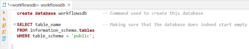
gapminder %>% write_rds(file = "./data/gapminder.rds")Using the SQL script shown in the screenshot below, a SQL database has been created called “workflowsdb”.
Using RPostgreSQL, the created datasets will be inserted into this database
(Creating a connection with SQL requires a password: in order to prevent the leakage of my password, the local RDS datafiles created above have been used instead of using the datafiles from an SQL database. The code which would be used if I were to use my password will still be shown)
source(here("R/login_credentials.R"))
con <- dbConnect(RPostgres::Postgres(),
                 dbname = "workflowsdb",
                 host = "localhost",
                 port = 5432,
                 user= "postgres",
                 password = rawToChar(pwd))

dbWriteTable(con, "gapminder", gapminder)
dbWriteTable(con, "dengue", dengue_separate)
dbWriteTable(con, "flu", flu_separate)
To inspect the database in order to check if all data has been transfered correctly, another SQL script has been used. Once again, screenshots of this script have been added underneath.
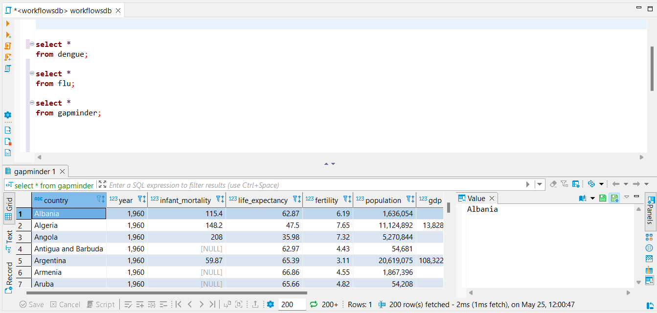
For further insurance, the data will also be inspected via R
source(here("R/login_credentials.R"))
con <- dbConnect(RPostgres::Postgres(),
dbname = "workflowsdb",
host = "localhost",
port = 5432,
user= "postgres",
password = rawToChar(pwd))
gapminder<-dbReadTable(con, "gapminder")
dengue<-dbReadTable(con, "dengue")
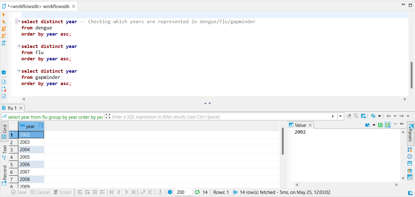
flu<-dbReadTable(con, "flu")We want to join the datasets based on “year” and on “countries”, thus we shall inspect those character vectors in partciular
list(gapminder_years=gapminder$year %>% unique(),
     dengue_years=dengue$year %>% unique(),
     flu_years=flu$year %>% unique())
## $gapminder_years
## [1] 1960 1961 1962 1963 1964 1965 1966 1967 1968 1969 1970 1971 1972 1973 1974 1975 1976 1977 1978 1979 1980 1981 1982 1983 1984 1985 1986 1987 1988 1989 1990
## [32] 1991 1992 1993 1994 1995 1996 1997 1998 1999 2000 2001 2002 2003 2004 2005 2006 2007 2008 2009 2010 2011 2012 2013 2014 2015 2016
##
## $dengue_years
## [1] 2002 2003 2004 2005 2006 2007 2008 2009 2010 2011 2012 2013 2014 2015
##
## $flu_years
## [1] 2002 2003 2004 2005 2006 2007 2008 2009 2010 2011 2012 2013 2014 2015Based on the years, we can state that dengue and flu share the same range of years, while gapminder has a way bigger range of years it covers
list(gapminder_countries=gapminder$country %>% unique %>% head(50),
     dengue_countries=dengue$country %>% unique,
     flu_countries=flu$country %>% unique)
## $gapminder_countries
## [1] Albania Algeria Angola Antigua and Barbuda Argentina Armenia
## [7] Aruba Australia Austria Azerbaijan Bahamas Bahrain
## [13] Bangladesh Barbados Belarus Belgium Belize Benin
## [19] Bhutan Bolivia Bosnia and Herzegovina Botswana Brazil Brunei
## [25] Bulgaria Burkina Faso Burundi Cambodia Cameroon Canada
## [31] Cape Verde Central African Republic Chad Chile China Colombia
## [37] Comoros Congo, Dem. Rep. Congo, Rep. Costa Rica Cote d'Ivoire Croatia
## [43] Cuba Cyprus Czech Republic Denmark Djibouti Dominican Republic
## [49] Ecuador Egypt
## 185 Levels: Albania Algeria Angola Antigua and Barbuda Argentina Armenia Aruba Australia Austria Azerbaijan Bahamas Bahrain Bangladesh Barbados ... Zimbabwe
##
## $dengue_countries
## [1] "Argentina" "Bolivia" "Brazil" "India" "Indonesia" "Mexico" "Philippines" "Singapore" "Thailand" "Venezuela"
##
## $flu_countries
## [1] "Argentina" "Australia" "Austria" "Belgium" "Bolivia" "Brazil" "Bulgaria" "Canada" "Chile"
## [10] "France" "Germany" "Hungary" "Japan" "Mexico" "Netherlands" "New.Zealand" "Norway" "Paraguay"
## [19] "Peru" "Poland" "Romania" "Russia" "South.Africa" "Spain" "Sweden" "Switzerland" "Ukraine"
## [28] "United.States" "Uruguay"In the countries, we can see a way wider spread of countries. Gapminder contains data of over 180 countries (only the top 50 are shown), while flu has 30 and dengue has 10. In order to create a full, properly joined dataset we will filter all 3 datasets to only contain shared years and shared countries
dengue_countries<-dengue$country %>% unique()
dengue_flu_countries<-flu$country %>% str_extract(pattern = dengue_countries) %>% unique() #Filtering for countries which
                                                                                      #are present in both dengue and flu
dengue_flu_countries<-dengue_flu_countries[!is.na(dengue_flu_countries)] #Filtering for NA's

gapminder$country %>% str_subset(pattern = dengue_flu_countries) %>% unique
## [1] "Argentina" "Brazil" "Mexico" "Bolivia"Based on these filters, the for countries available in every dataset are: Argentina, Brazil, Mexico, Bolivia
flu_year<-flu$year

gapminder_join<-gapminder %>% filter(year <= max(flu_year) & year >=min(flu_year)) %>%
  filter(country %in% dengue_flu_countries)

data_full<-left_join(gapminder_join, dengue, by = c("country", "year")) %>%
  left_join(flu, by = c("country", "year", "month", "day"))
Now, with this fully joined dataset filtered for both mutual countries and years, some visualisations will be performed
Firstly, dengue incidence in 4 countries over 15 years
data_sum_dengue<-data_full %>% group_by(country, year) %>%
  dplyr::summarise(mean=mean(dengue_incidence, na.rm=TRUE))
## `summarise()` has grouped output by 'country'. You can override using the `.groups` argument.data_sum_dengue %>% ggplot(aes(x=year, y=mean))+
geom_point(aes(color = country))+
geom_line(aes(color = country))+
labs(
title="Dengue incidence over 12 years in 4 countries",
x="Time in years",
y="incidence (unit not mentioned)"
)+
theme_bw()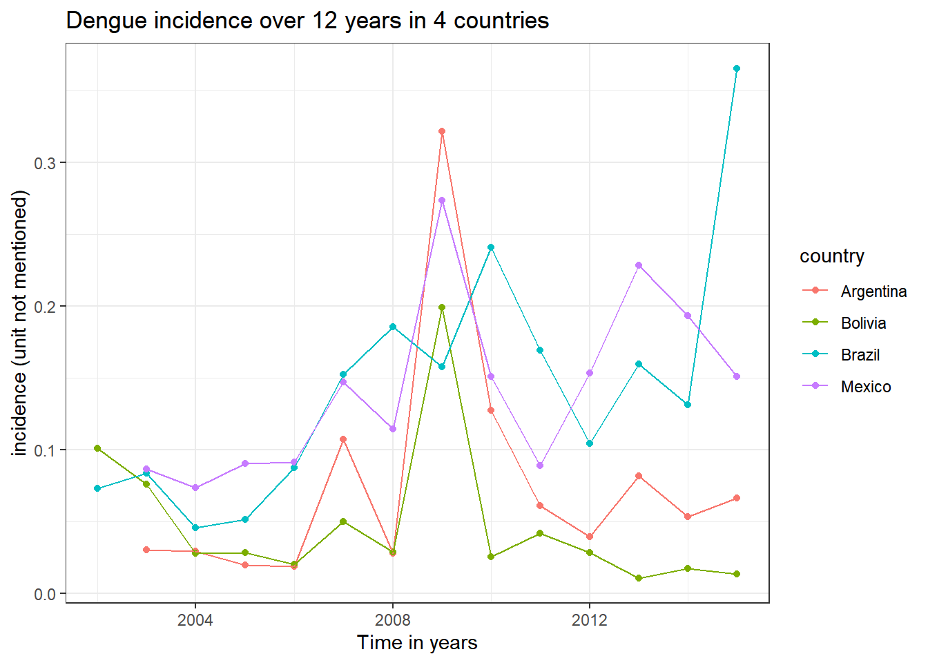
Secondly, the incidence of flue through the months in the 4 different countries
month_data<-data.frame(
  month=seq(1:12),
  MONTH=c("January", "Februari", "March", "April", "May", "June", "July",
          "August", "September", "October", "November", "December")
)

month_data$MONTH<-factor(month_data$MONTH, levels =c("January", "Februari", "March", "April", "May", "June", "July",
                                                     "August", "September", "October", "November", "December"))

data_month<-left_join(data_full, month_data, by="month")

data_month %>% ggplot(aes(x=MONTH, y=flu_incidence))+
  geom_col(aes(fill=country), position = position_dodge())+
  labs(
    title="Flu incidence by month in 4 countries",
    x="Month",
    y="Incidence (unit not mentioned)"
  )+
  theme_bw()+
  theme(axis.text.x = element_text(angle=45, hjust=1))
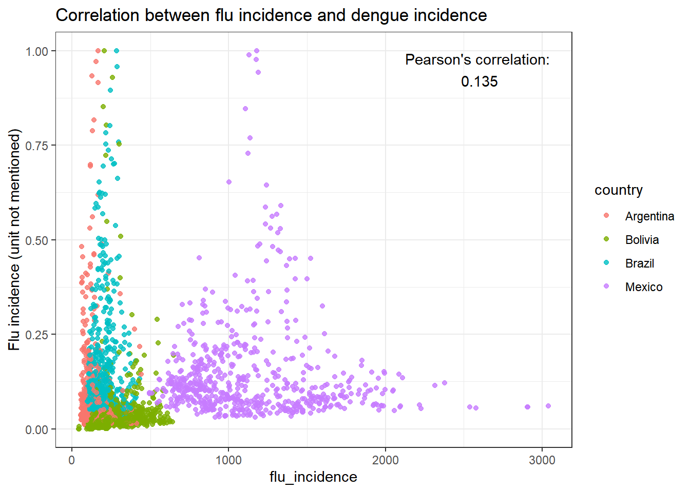
And finally, a correlation between dengue incidence and flu incidence? (Spoiler: no. Not at all.)
correlation<-cor.test(data_full$dengue_incidence, data_full$flu_incidence, method=c("pearson"))$estimate %>%
  round(digits = 3)

data_full %>% ggplot(aes(x=flu_incidence, y=dengue_incidence))+
  geom_point(aes(color=country), alpha = 0.8)+
  labs(
    title="Correlation between flu incidence and dengue incidence",
    y="Flu incidence (unit not mentioned)",
    y="Dengue incidence (unit not mentioned"
  )+
  annotate("text", x=2600, y=0.95, label = paste0("Pearson's correlation: \n", correlation))+
  theme_bw()