Random forest in Glass

Frontpage Data visualisation Parametizing data Directory structure R-package SQL Zotero Reproductibility Future endeavours Free research (Machine learning) CV Bibliography

Perfoming the entire randomForest workflow on the glass dataset

library(mlbench)
data(Glass)

set.seed(4321)
ind_glass<-sample(2, nrow(Glass), replace=TRUE, prob=c(0.67,0.33)) #Creating a random selection of datapoints

glass_training<-Glass[ind_glass==1,] # Separating the training the training and the testing datasets
glass_test<-Glass[ind_glass==2,]

knitr::kable(summary(glass_training))

RI	Na	Mg	Al	Si	K	Ca	Ba	Fe	Type
Min. :1.511	Min. :11.02	Min. :0.000	Min. :0.290	Min. :69.89	Min. :0.0000	Min. : 5.430	Min. :0.0000	Min. :0.00000	1:49
1st Qu.:1.517	1st Qu.:12.89	1st Qu.:2.703	1st Qu.:1.190	1st Qu.:72.33	1st Qu.:0.1375	1st Qu.: 8.295	1st Qu.:0.0000	1st Qu.:0.00000	2:50
Median :1.518	Median :13.28	Median :3.475	Median :1.345	Median :72.80	Median :0.5600	Median : 8.615	Median :0.0000	Median :0.00000	3:13
Mean :1.518	Mean :13.42	Mean :2.819	Mean :1.425	Mean :72.70	Mean :0.4599	Mean : 8.830	Mean :0.1589	Mean :0.05708	5: 7
3rd Qu.:1.519	3rd Qu.:13.78	3rd Qu.:3.592	3rd Qu.:1.583	3rd Qu.:73.07	3rd Qu.:0.6000	3rd Qu.: 9.062	3rd Qu.:0.0000	3rd Qu.:0.09000	6: 7
Max. :1.534	Max. :17.38	Max. :4.490	Max. :3.500	Max. :75.41	Max. :2.7000	Max. :16.190	Max. :2.2000	Max. :0.51000	7:18

knitr::kable(summary(glass_test))

RI	Na	Mg	Al	Si	K	Ca	Ba	Fe	Type
Min. :1.513	Min. :10.73	Min. :0.000	Min. :0.470	Min. :69.81	Min. :0.0000	Min. : 6.470	Min. :0.0000	Min. :0.00000	1:21
1st Qu.:1.516	1st Qu.:12.96	1st Qu.:0.000	1st Qu.:1.173	1st Qu.:72.20	1st Qu.:0.1100	1st Qu.: 8.180	1st Qu.:0.0000	1st Qu.:0.00000	2:26
Median :1.518	Median :13.32	Median :3.495	Median :1.410	Median :72.78	Median :0.5500	Median : 8.595	Median :0.0000	Median :0.00000	3: 4
Mean :1.519	Mean :13.38	Mean :2.408	Mean :1.486	Mean :72.55	Mean :0.5734	Mean : 9.218	Mean :0.2083	Mean :0.05686	5: 6
3rd Qu.:1.521	3rd Qu.:13.91	3rd Qu.:3.607	3rd Qu.:1.695	3rd Qu.:73.10	3rd Qu.:0.6175	3rd Qu.: 9.640	3rd Qu.:0.0000	3rd Qu.:0.10000	6: 2
Max. :1.531	Max. :15.15	Max. :3.900	Max. :3.040	Max. :73.75	Max. :6.2100	Max. :14.680	Max. :3.1500	Max. :0.37000	7:11

ModelGlass<-randomForest::randomForest(Type ~ ., data=glass_training, importance = TRUE)

PredictGlass<-predict(ModelGlass, glass_test, type="class")
table(PredictGlass, glass_test$Type)

##             
## PredictGlass  1  2  3  5  6  7
##            1 19  0  3  0  0  0
##            2  2 23  0  3  1  1
##            3  0  1  1  0  0  0
##            5  0  2  0  3  0  0
##            6  0  0  0  0  1  0
##            7  0  0  0  0  0 10

importance(ModelGlass)

##             1         2          3           5          6          7 MeanDecreaseAccuracy MeanDecreaseGini
## RI 25.9516672 15.981884  8.6355170  3.01558132  5.2054141  8.1761219            28.527676        14.982608
## Na  7.0153218  3.465588  2.4742629  2.67561186 10.7079299  9.5412346            14.240678         8.973814
## Mg 20.7226854 18.360376 12.0696619 15.77226943 12.9410416 16.0526327            32.439182        17.157482
## Al 20.7919497 20.688041  7.8135932 11.89337555  0.4693794 15.1221411            30.049922        16.833501
## Si 11.3400744  2.932622  3.0995611 -0.07519902  4.6446785  2.7584307            12.602525         7.992729
## K   9.5158955 11.211496  5.0377273  2.96884643 14.7675552  7.7917593            17.856605        10.573783
## Ca 13.3933883 23.812395  5.5731976 11.54097673  2.0839665  5.9300857            28.135538        15.254431
## Ba  4.2571321 13.147049  4.7544812  3.80935388  6.1771571 26.1962433            24.494792         9.858269
## Fe  0.1021816  2.533907  0.7303576 -2.90363006  3.8284240  0.6368166             2.003686         3.380027

varImpPlot(ModelGlass)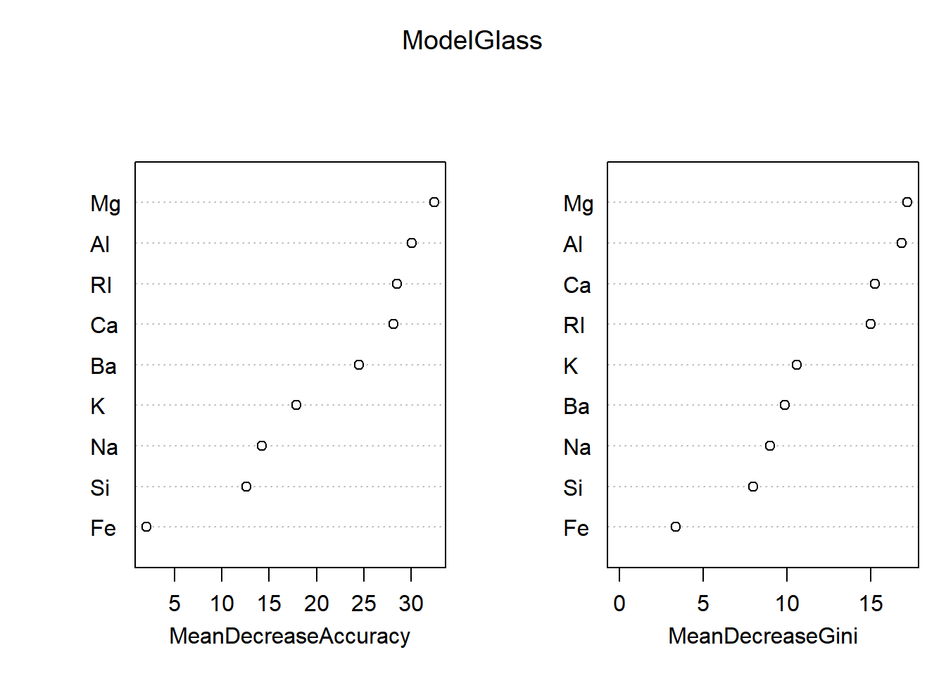

confusionMatrix(PredictGlass, glass_test$Type)

## Confusion Matrix and Statistics
## 
##           Reference
## Prediction  1  2  3  5  6  7
##          1 19  0  3  0  0  0
##          2  2 23  0  3  1  1
##          3  0  1  1  0  0  0
##          5  0  2  0  3  0  0
##          6  0  0  0  0  1  0
##          7  0  0  0  0  0 10
## 
## Overall Statistics
##                                           
##                Accuracy : 0.8143          
##                  95% CI : (0.7034, 0.8972)
##     No Information Rate : 0.3714          
##     P-Value [Acc > NIR] : 3.969e-14       
##                                           
##                   Kappa : 0.7406          
##                                           
##  Mcnemar's Test P-Value : NA              
## 
## Statistics by Class:
## 
##                      Class: 1 Class: 2 Class: 3 Class: 5 Class: 6 Class: 7
## Sensitivity            0.9048   0.8846  0.25000  0.50000  0.50000   0.9091
## Specificity            0.9388   0.8409  0.98485  0.96875  1.00000   1.0000
## Pos Pred Value         0.8636   0.7667  0.50000  0.60000  1.00000   1.0000
## Neg Pred Value         0.9583   0.9250  0.95588  0.95385  0.98551   0.9833
## Prevalence             0.3000   0.3714  0.05714  0.08571  0.02857   0.1571
## Detection Rate         0.2714   0.3286  0.01429  0.04286  0.01429   0.1429
## Detection Prevalence   0.3143   0.4286  0.02857  0.07143  0.01429   0.1429
## Balanced Accuracy      0.9218   0.8628  0.61742  0.73438  0.75000   0.9545

Without editing the mtry and ntree, we get a accuracy of ~ 0.81 (which, mind you, is already way higher than the original accuracy of ~ 0.7 given by the KKN model). Now we’ll test for the optimum mtry and kmean amount again, like with the cars dataset.

x=c()
for(i in 1:9){
  Model3<-randomForest(Type ~ ., data= glass_training, ntree = 500, mtry = i, importance = TRUE)
  PredictModel3<-predict(Model3, glass_training, type="class")
  x[i]=mean(PredictModel3 == glass_training$Type)
}
data.frame(mtry=1:9,
           prediction_power=x)

##   mtry prediction_power
## 1    1                1
## 2    2                1
## 3    3                1
## 4    4                1
## 5    5                1
## 6    6                1
## 7    7                1
## 8    8                1
## 9    9                1

Conclusion: any mtry above 1 is good enough

y=c()

length<-c(1 %o% 10^(0:4))
for(i in c(1 %o% 10^(0:4))){
  Model3<-randomForest(Type ~ ., data= glass_training, ntree = i, mtry = 6, importance = TRUE)
  PredictModel3<-predict(Model3, glass_training, type="class")
  y[i]=(mean(PredictModel3 == glass_training$Type))
}
data<-data.frame(prediction_power=y[length],
                 ntree=length)
data

##   prediction_power ntree
## 1        0.8402778     1
## 2        0.9791667    10
## 3        1.0000000   100
## 4        1.0000000  1000
## 5        1.0000000 10000

Once again, any amount of Ntree above 1 is good enough

Based on these results, we can see that changing the mtry/ntree will not affect the data in any mayor way. However, to see if this hypothesis is truly true, we’ll test it anyway.

ModelGlass<-randomForest::randomForest(Type ~ ., data=glass_training, ntree = 1000, mtry = 3, importance = TRUE)

PredictGlass<-predict(ModelGlass, glass_test, type="class")
table(PredictGlass, glass_test$Type)

##             
## PredictGlass  1  2  3  5  6  7
##            1 19  0  3  0  0  0
##            2  2 23  0  1  1  1
##            3  0  1  1  0  0  0
##            5  0  2  0  5  0  0
##            6  0  0  0  0  1  0
##            7  0  0  0  0  0 10

importance(ModelGlass)

##             1         2          3          5          6         7 MeanDecreaseAccuracy MeanDecreaseGini
## RI 35.9425852 22.955617 12.6393173  3.2609681  8.0461891 10.125891            39.452868        15.374026
## Na 12.6946465  5.804545  2.7151993  9.8071309 12.1866461 13.824966            19.901691         8.870768
## Mg 31.4568425 23.237537 13.5906352 20.4221998 17.8087921 22.382001            43.929844        17.504698
## Al 31.3450931 30.832605 10.5723607 17.2216312  0.1824541 19.557992            44.152502        17.547209
## Si 19.5356383  4.501227  5.6543712  0.5365142  5.1377628  3.770462            20.553736         8.018075
## K  15.8786105 14.925417  5.7598017  2.2652263 19.8542689 10.047250            26.789079        10.013021
## Ca 16.3234783 32.337265  7.1320768 16.6442932  3.1952506  9.074469            36.829526        15.234269
## Ba  7.2861647 15.662737  6.3118076  4.0829257  7.0805242 39.179560            35.069476         9.358338
## Fe -0.8240873  3.557017  0.7700442 -3.5323248  5.3702326  1.195446             2.635895         3.208900

varImpPlot(ModelGlass)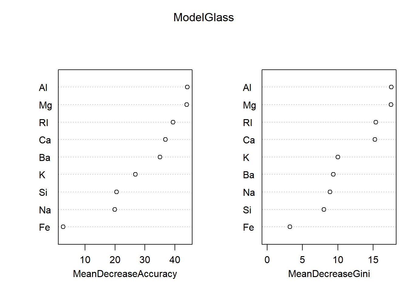

confusionMatrix(PredictGlass, glass_test$Type)

## Confusion Matrix and Statistics
## 
##           Reference
## Prediction  1  2  3  5  6  7
##          1 19  0  3  0  0  0
##          2  2 23  0  1  1  1
##          3  0  1  1  0  0  0
##          5  0  2  0  5  0  0
##          6  0  0  0  0  1  0
##          7  0  0  0  0  0 10
## 
## Overall Statistics
##                                           
##                Accuracy : 0.8429          
##                  95% CI : (0.7362, 0.9189)
##     No Information Rate : 0.3714          
##     P-Value [Acc > NIR] : 6.15e-16        
##                                           
##                   Kappa : 0.783           
##                                           
##  Mcnemar's Test P-Value : NA              
## 
## Statistics by Class:
## 
##                      Class: 1 Class: 2 Class: 3 Class: 5 Class: 6 Class: 7
## Sensitivity            0.9048   0.8846  0.25000  0.83333  0.50000   0.9091
## Specificity            0.9388   0.8864  0.98485  0.96875  1.00000   1.0000
## Pos Pred Value         0.8636   0.8214  0.50000  0.71429  1.00000   1.0000
## Neg Pred Value         0.9583   0.9286  0.95588  0.98413  0.98551   0.9833
## Prevalence             0.3000   0.3714  0.05714  0.08571  0.02857   0.1571
## Detection Rate         0.2714   0.3286  0.01429  0.07143  0.01429   0.1429
## Detection Prevalence   0.3143   0.4000  0.02857  0.10000  0.01429   0.1429
## Balanced Accuracy      0.9218   0.8855  0.61742  0.90104  0.75000   0.9545

Specifying the ntree to 1000 and mtry to 3 gives a small increase in accuracty, up to ~ 0.82.

With this, I’ve proven my skills in setting up a randomForest machine learning algorythm for a dataset, and performing small-scale optimisations to the algorythm. Next, as final research subject, we’ll move on to a randomForest-based machine learning technique specifically made for micriology: IDTAXA